Particle tracking SUNTANS velocity data

Particle tracking is performed using the suntrack.py module.

This tutorial is in the headland SUNTANS example.

Running the particle tracking code

This code can be found here.

First import the SunTrack and GridParticles module and set some variables:

    from suntrack import SunTrack, GridParticles
    import numpy as np

    ########
    # Inputs
    ncfile = 'data/Headland_0*.nc'

    outfile = 'data/Headland_particles.nc'

    timeinfo = ('20130101.0200','20130102.0820',120.0)

    dtout = 600.

    dx = 100.   
    dy = 100.

    # Grid parameters
    W = 2.5e4
    a =2e3
    b =8e3
    x0 = 0

    ########

Then use the GridParticles function to allocate the particle locations within the grid.

    # Polygon to fill with particles
    XY = np.array([
        [x0-W/2, 0],\
        [x0-W/2, 2*b],\
        [x0+W/2, 2*b],\
        [x0+W/2, 0],\
        [x0-W/2, 0],\
        ])

    x,y,z = GridParticles(ncfile,dx,dy,1,xypoly=XY) 

Alternatively, a polygon can be read in from a shape file with something like this:

    from maptools import readShpPoly

    polyfile = '/path/to/a/polygon_shapefile.shp'
    XY,newmarker = readShpPoly(polyfile,FIELDNAME=None )

    # XY is a list of polygons stored as numpy arrays (N,2)
    XY = XY[0] # use the first polygon stored in the shapefile

Initialize the particle tracking object.

• set "is3D = True" to track in 3D, else use surface layer velocity only.

    sun = SunTrack(ncfile, interp_method='mesh', interp_meshmethod='nearest',
        is3D=False)

Once the object is initialized, it can be called using different start locations and/or start times. It is called using

    sun(x,y,z,timeinfo,agepoly=agepoly,outfile=outfile,dtout=dtout)

The particle locations (x, y, z) are then save to outfile at every dtout seconds.

Visualizing the output

This example shows how to create an animation of particle pathlines similar to this example:

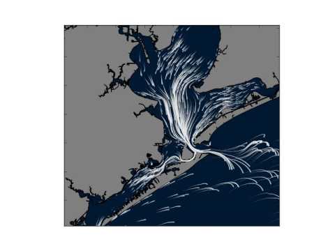
The code for the headland case can be found here..

First, import the relevant libraries:

    from suntrack import PtmNC
    import matplotlib.pyplot as plt
    import numpy as np

    import matplotlib.animation as animation
    from otherplot import streakplot
    from maptools import plotmap

    ###########
    # Inputs
    ncfile = 'data/Headland_particles.nc'
    outfile = 'plots/Headland_particle_streak.mov'

    taillength = 18 # Number of time steps for tail
    subset = 60 # Only plot every nth particle

    # Plot specific stuff
    #shpfile= '../../DATA/GalvestonBasemapCoarse.shplocations
    W = 2.5e4
    a =2e3
    b =8e3
    x0=0

    xlims = [x0-W/2, x0+W/2]
    ylims = [0, 2*b]
    ###########

The class for handling the particle NetCDF output files is called PtmNC. The code for making the pretty streaks is in a function called streakplot that is in the otherplot.py package.

The particle file object is initialized and the first few time steps are read in

    # Itialize the particle class
    sun = PtmNC(ncfile)

    tstart = range(0,sun.nt-taillength)
    ts = range(tstart[0],tstart[0]+taillength)

    # Read the particle locations at the initial step
    xp = sun.read_step(ts,'xp')[::subset,:]
    yp = sun.read_step(ts,'yp')[::subset,:]
    zp = sun.read_step(ts,'zp')[::subset,:]

then the first step is plotted:

    # Plot specific stuff
    fig,ax = plt.subplots()
    ax.set_axis_bgcolor('#001933')
    ax.set_xticklabels([])
    ax.set_yticklabels([])

    # This plots a map
    #plotmap(shpfile)

    # Initialize the streak plot
    S=streakplot(xp,yp,ax=ax,xlim=xlims,ylim=ylims)

Finally, the following code generates an animation:

    ####
    # Animation code
    ####

    def updateposition(i):
        print i
        ts = range(tstart[i],tstart[i]+taillength)
        xp = sun.read_step(ts,'xp')[::subset,:]
        yp = sun.read_step(ts,'yp')[::subset,:]

        S.update(xp,yp)

        return S.lcs

    anim  = animation.FuncAnimation(fig,updateposition,frames=len(tstart),\
        interval=50,blit=True)

    print 'Building animation...'
    anim.save(outfile,fps=6,bitrate=3600)
    print 'Done'